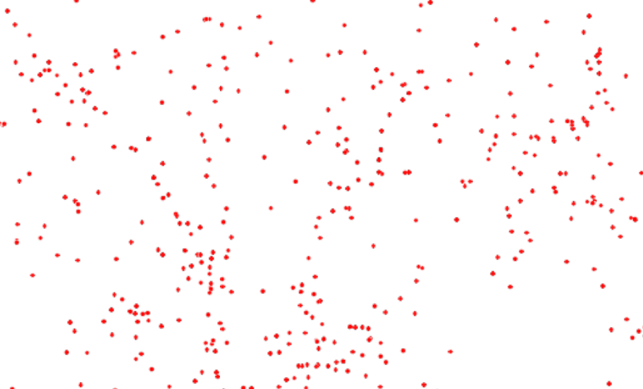
When modeling the spatial distribution of physical phenomena such as elevation, soil properties, strata thickness etc. from a measured set of discrete points such as in the image above, a question often arises as to what interpolation method to use. The points may be sparse and irregular, or dense and regularly spaced, but the interpolation methods usually assume the variable being modeled, elevation for example, is continuous across the study area. The goal is to create an even grid of data points in the study area by predicting and filling-in data at unsampled points. In general spatial interpolation will accomplish the following:
-
Convert a sample of data points to a complete coverage (set of values) for the study region.
-
Convert from one level of data resolution or orientation to another (resampling). Usually resolution is reduced to the coarsest in a set, but resolution can be increased using a suitable interpolator, such as a simple or incremental bicubic spline (stair interpolation).
-
Convert from one representation of a continuous surface to another, e.g. TIN to grid or contour to grid.
There are many interpolation and approximation methods developed to calculate and predict the missing values. The models may go precisely through the sample point i.e. the modeled value is exactly equal to the sampled value or may approximate values at the sample points i.e. the modeled values is close but not equal to the sampled value.
The image below shows that there is no unique solution. Different functions will track different lines as they approximate the data at unsampled points—interpolating or extrapolating to generate values where data is missing.
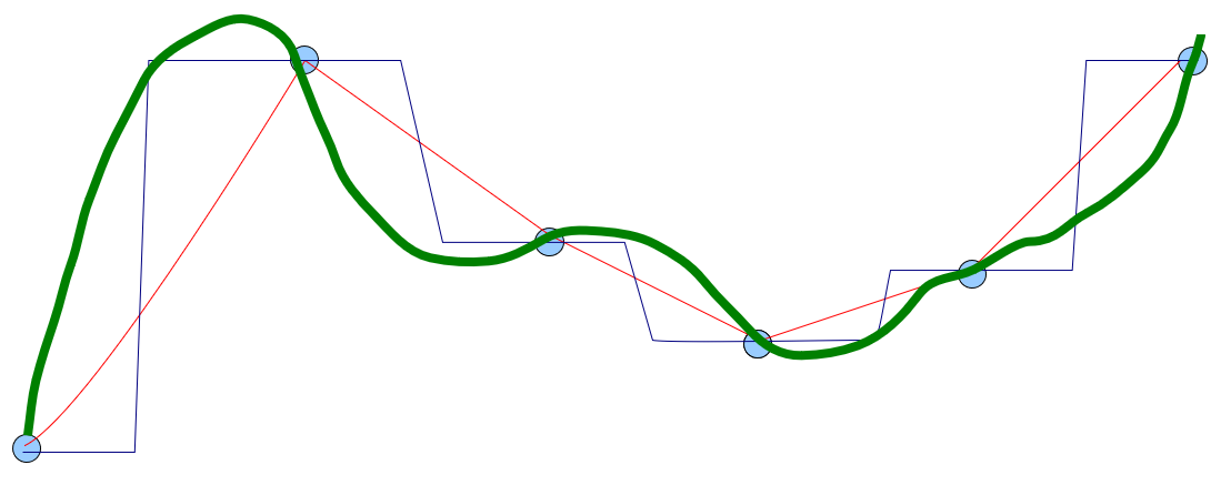
Source: Helena Mitasova - Geospatial Analysis and Modeling MEA592
Many studies compare interpolation techniques using a range of datasets and conditions, and there are some well-defined factors that have a major influence on the quality of the interpolation: data measurement accuracy, data density, data distribution, and spatial variability 1
Whereas there is no one best gridding method for a particular type of data, experience and the data itself helps in selecting a method that will best represent the output for the intended use. One way is to compare the predicted value in the model at a point with an actual measurement taken at the same point from the field. The closer the two values are to each other, the better the selected interpolation method models the particular dataset. If this testing is repeated, we can add up all the errors(residuals) and make a determination of the effectiveness of one model against another. An example of a variable that could be treated in this manner is the thickness of a given strata e.g. limestone, coal etc.
In Carlson, there is a way to check the accuracy of a selected modeling method in predicting values at unsampled points without going to field to take actual measurements. We can, for example, take 30 sample points and model with 29 and then check the error residual at the removed sample point. By repeating this removal process across all 30 sample points and verifying the average residual error and the standard deviation of the residual error we can decide on the most suitable method to model a dataset.
Modeling methods available in Carlson include:
- Triangulation
- Inverse Distance
- Kriging
- Polynomial
- Linear least squares
- ABOS Method
- Voronoi
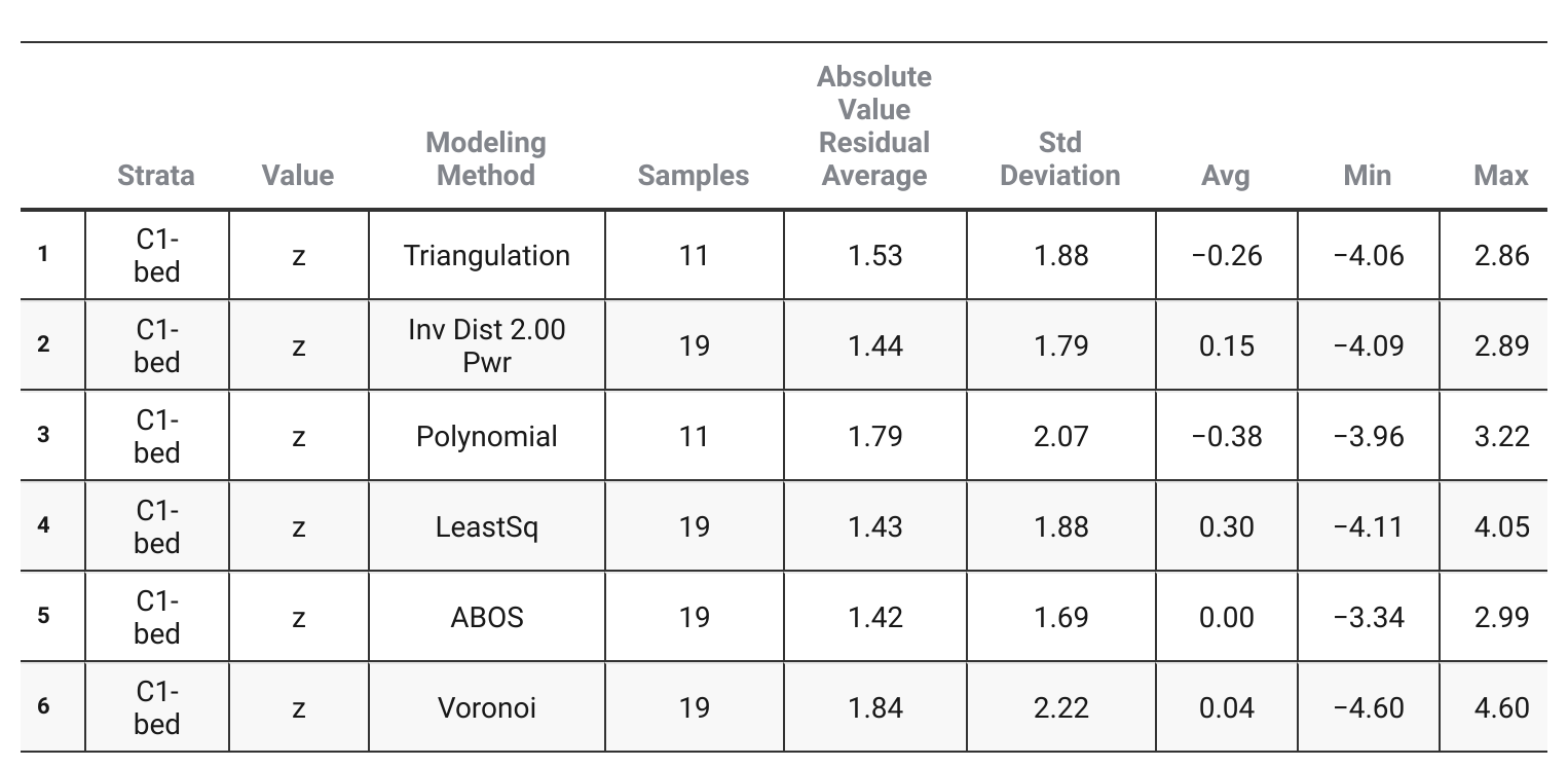
The table below compares six of the methods available in Carlson on the same dataset. The output shows ABOS has the lowest standard deviation and absolute value residual average. It is therefore, the best modeling method for the dataset studied here.
All interpolation methods in Carlson or when implemented in other systems such as surfer, ArcGIS etc., have options and parameters that must be adjusted to generate models that approximate the data as much as possible. The process may include trial and error, but with experience and repeated use, it is clear which methods work best for what data set.
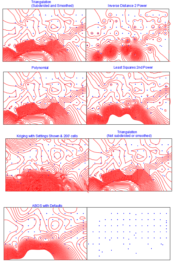
The contour plots generated in the figure below illustrate how different interpolation methods may model the same dataset.
- Inverse Distance with 2nd Power
- Polynomial
- Lease Squares with 2nd Power
- Kriging
- Triangulation without Subdivision or Smoothing
- ABOS
-
] Geospatial Analysis 6th Edition - MF Goodchild ↩︎